 Freedom Calcs
Withdrawal assumptions
The 4% Rule Has 9 Assumptions to Check. Here's What Can Break.
Check the 4% rule's assumptions about time, portfolios, inflation, fees and US history, with reproducible examples of sequence risk and a nine-point checklist.
The short answer
The 4% rule starts withdrawals at 4% of your initial portfolio, then adjusts that dollar amount for inflation. Its historical support depends on the horizon, investments and spending method tested. It does not guarantee future income. Check nine conditions before applying it, especially early losses, costs and whether US market history fits your plan.
What the 4% rule actually says
A $1 million starting portfolio gives a $40,000 first withdrawal under the 4 percent rule. After an assumed 3% inflation adjustment, the next withdrawal is $41,200. Recalculating 4% of the remaining account each year creates a different strategy.
For the basic formula, read how the 4 percent rule works. This article examines when applying it becomes unreliable. Some of the nine checks concern the original research design; others concern assumptions people add when turning research into a household budget.
Bengen’s 1994 paper studied historical US returns and inflation, including difficult sequences. His roughly 4% finding addressed a minimum 30-year planning horizon under the conditions examined. It was never based on smooth returns or steady inflation.
The calculations below separate three jobs: historical evidence, hypothetical retirement withdrawals, and the site’s retirement-target arithmetic. A calculator result can answer only the questions its model supports.
Assumption 1: Your planning horizon fits the evidence
Retiring at 65 and planning through 95 requires 30 years. Starting at 50 with the same endpoint requires 45. A withdrawal rate tested over one horizon does not automatically transfer to the other. A surviving partner may also need income after the first household death.
There is no universal safe withdrawal rate by age. Age helps define the horizon, but investments, expenses and the spending policy still matter. Consider $1 million earning exactly zero after inflation, with no taxes or fees:
| Years funded | Annual spending in today’s dollars | Starting balance divided by years |
|---|---|---|
| 30 | $33,333 | 3.33% |
| 35 | $28,571 | 2.86% |
| 40 | $25,000 | 2.50% |
| 45 | $22,222 | 2.22% |
Calculated October 28, 2026: annual spending = $1,000,000 ÷ years, with unrounded values used internally. The balance is exhausted after the final withdrawal. These are arithmetic spending limits under a zero-return assumption, not safe rates inferred from markets.
At $40,000 annually, the same zero-real-return balance funds 25 withdrawals. The Coast FIRE calculator lets you change the retirement starting age and chosen withdrawal rate to examine the savings target. It does not model years spent in retirement. If your horizon exceeds the evidence, the withdrawal policy needs a separate longer-horizon test.
Assumption 2: Your portfolio resembles the investments tested
The 1998 Trinity study’s methods specify five stock allocations: 100%, 75%, 50%, 25% and 0%; the remainder was bonds. It used S&P 500 stocks and long-term high-grade corporate bonds. Bengen’s core analysis used intermediate-term Treasuries instead, so even these studies have different bond exposures.
What if you hold 30% stocks? That allocation was not a Trinity test row. Interpolating a personal success probability between two rows would hide how returns interact with withdrawals. A lower stock weight can reduce some market swings while leaving less growth to finance a long retirement.
Write down what you own, including concentration and bond duration. A portfolio dominated by one employer’s shares, cash or speculative assets does not inherit the research merely because its starting withdrawal is 4%. Also record the rebalancing policy you can follow. An allocation that drifts after a crash can become a different experiment from the one you meant to copy.
If your holdings differ substantially, use research or a withdrawal model that actually represents them before treating its results as relevant.
Assumption 3: Sequence of returns risk fits inside your plan
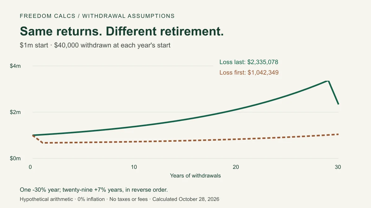
Two portfolios can receive exactly the same annual returns and still fund withdrawals differently. Consider two hypothetical retirees who each start with $1 million and withdraw $40,000 at the beginning of every year. Inflation, taxes and fees are zero, so the withdrawal also stays constant in purchasing power.
Each experiences one −30% year and twenty-nine +7% years. The only change is order: the loss comes first for one retiree and last for the other. Both have an arithmetic average return of 5.77% and a compound annual return of about 5.50% before withdrawals.
| End of year | Loss first | Loss last |
|---|---|---|
| 1 | $672,000 | $1,027,200 |
| 5 | $690,825 | $1,156,420 |
| 10 | $722,787 | $1,375,807 |
| 20 | $830,487 | $2,115,077 |
| 30 | $1,042,349 | $2,335,078 |
Calculated October 28, 2026 using the recurrence below, without rounding intermediate balances. Both fund all 30 withdrawals. The final difference is $1,292,729; this example illustrates a smaller remaining cushion, rather than a failure in either path.
End balance = (previous balance − $40,000) × (1 + that year's return)
Loss-first year 1 = ($1,000,000 − $40,000) × 0.70 = $672,000
Loss-last year 1  = ($1,000,000 − $40,000) × 1.07 = $1,027,200
Repeat for all 30 years, moving the −30% year from first to last.
Without withdrawals, reversing these returns leaves the final value unchanged. With withdrawals, early losses reduce the capital available to compound while spending continues. Comparing only average returns misses that cash-flow interaction.
The original studies already incorporated varying historical returns, including sequence of returns risk. The unsupported assumption is that your future sequence will be adequately represented by the sequences tested, or that a smooth projection can replace them. These invented returns establish no failure probability and no historically safe rate.
Check our withdrawal assumptions before using the Coast FIRE calculator: it models accumulation with a constant return. Changing that one return input cannot recreate these two withdrawal paths. If a plan relies on the average to rescue early losses, examine an actual retirement withdrawal schedule and the spending changes you could make during those years.
Assumption 4: The inflation adjustment matches your costs
At constant hypothetical 3% inflation, a $40,000 first withdrawal becomes $52,191 in year ten. At 6%, it becomes $67,579. Each maintains the same purchasing power under its own assumed price path; the nominal cash requirement differs considerably.
The original inflation-adjusted method used changing historical prices. It did not assume that inflation stayed steady, and difficult inflation episodes were part of the evidence. To inspect price history, use FRED’s BLS CPI series, specifying the observation frequency and comparison dates. Monthly year-over-year changes and annual-average changes answer different questions.
Trinity’s method also decreased withdrawals during deflation. For illustration, a 2% decrease turns $40,000 into $39,200. Refusing that cut introduces a nominal spending floor and changes the policy being tested.
Your own bills may behave differently. The BLS explains CPI’s coverage; it is an aggregate measure. A rent reset, insurance premium or care bill can outrun that adjustment. If personal costs rise faster, the planned withdrawal buys less than your budget requires.
Assumption 5: You follow the spending rule you selected
Suppose the portfolio falls to $700,000 before a new withdrawal is set. Taking 4% of that balance produces $28,000. Continuing a $40,000 initial withdrawal after 3% inflation produces $41,200. Those policies deliver different incomes and leave different amounts invested.
A fixed percentage of current assets responds automatically to market value. Its weakness for a household is the possibility of a substantial income cut. Maintaining a fixed real dollar withdrawal supports steadier purchasing power while asking more of the portfolio during declines.
Guardrails introduce rules for adjusting spending when specified conditions are met. Variable percentage withdrawal, or VPW, recalculates a spending percentage using a defined framework. Neither label makes a withdrawal sustainable by itself: the parameters and permitted cuts determine what the household must tolerate.
Before comparing flexible methods, write down the minimum spending you can accept and which expenses can move. Our methodology’s withdrawal section explains the narrower target calculation used here. It does not implement a guardrails or VPW strategy. If you change policies after losses, an earlier result for fixed spending no longer describes the plan you are following.
Assumption 6: Portfolio-funded spending is complete
The rule concerns withdrawals from investments. It does not require investments to be your only income source. Social Security, a pension, rental income or work can reduce the amount the portfolio must provide, if amounts and timing match the budget.
For a hypothetical $60,000 annual budget and $20,000 of continuing income available immediately, the gap is $40,000. Dividing by 4% gives $1 million. If the income begins ten years later, that subtraction leaves the first decade unfunded; plan the bridge separately.
Use consistent tax treatment. A gross pension does not necessarily offset the same amount of after-tax spending. Rent also needs an allowance for operating costs and vacancies before you treat it as available income.
The FIRE Number calculator checks the target for a specified spending gap. Compare a higher budget in the Fat FIRE calculator or a constrained essential budget in Lean FIRE, without assuming the label determines a withdrawal rate.
Keep irregular needs visible: a replacement roof or family assistance can require withdrawals beyond the annual allowance. An incomplete spending gap understates the target even when the division is correct.
Assumption 7: Costs and taxes fit inside the budget
Trinity excluded taxes and transaction costs. The SEC explains how fees reduce the amount left earning returns. Here is a separate accumulation example using this site’s actual Coast calculation engine.
Set age 35, retirement age 65, assets $1 million, annual spending $40,000, monthly contributions $0, inflation 3% and withdrawal assumption 4%. Change only the nominal return:
| Annual nominal return | Nominal value after 30 years | Value in today’s dollars |
|---|---|---|
| 7.00% | $7,612,255 | $3,136,148 |
| 6.00% | $5,743,491 | $2,366,242 |
| 5.93% | $5,630,788 | $2,319,810 |
Calculated October 28, 2026. No withdrawals occur in this comparison. The first two rows model a one-percentage-point return drag. An exact 1% charge on each year’s post-growth balance instead gives 1.07 × 0.99 − 1 = 5.93%, shown separately. Nominal values follow $1,000,000 × (1 + return)^30; today’s-dollar values divide by 1.03^30. See how returns are compounded.
Count expenses already reflected in quoted returns only once. Taxes also affect the cash you retain from a withdrawal; the amount depends on the account. If costs sit outside your spending and return assumptions, a seemingly adequate gross withdrawal can leave a household short.
Assumption 8: US market history fits the retirement you are funding
A US historical result does not establish a universally safe rate. Wade Pfau’s 2010 international study examined 17 developed countries using data from 1900 through 2008 and 30-year retirements beginning from 1900 through 1979. It considered domestic investments and local inflation.
Even with an optimistic assumption that selected the best fixed allocation for each retirement using hindsight, 4% survived every tested retirement in only four countries. Table 3 includes historical failures in Japan, Germany and Italy. Those results challenge treating the US experience as a universal floor.
Read the assumptions around that table. Its allocations benefit from information a retiree would not have had. Its domestic portfolios are not a present-day globally diversified portfolio. In a separate fixed 50/50 analysis, the paper reports historical failures somewhere in the sample for all 17 countries, including the US. Different datasets and allocations can change even the US result.
For your own plan, separate investment geography from spending currency. A person spending yen while holding US assets has a currency exposure that a purely US-dollar example does not show. A dollar withdrawal target cannot, on its own, specify the number of yen available for groceries.
Consider a hypothetical household that holds the same investments before and after moving abroad. Its portfolio statement may be unchanged in dollars, while its local spending requirement changes with exchange rates. Lowering a return input is a rough sensitivity exercise; it does not model the currency path or the timing of local bills.
China was not in this study’s 17-country sample. It would be unsupported to claim that this paper proves a particular failure rate for Chinese retirees. Equally, a Japanese historical failure is not evidence that every Japanese household today needs the same rate. An internationally diversified account, pension income and a different spending policy each pose another test.
If your market exposure or spending currency differs from the evidence, record that mismatch explicitly. Look for a withdrawal analysis that matches those features before importing a US percentage into the budget. Geographic limits belong beside the result because they change what the result can tell you.
Assumption 9: You can maintain the plan through a severe decline
Imagine a $1 million portfolio falling 40% to $600,000 before the next withdrawal. A planned $40,000 payment is now 6.67% of the remaining assets, even though its initial rate was 4%. That larger current-balance percentage follows from the same spending rule.
The arithmetic does not tell you whether you would keep the allocation, cut spending or sell investments after seeing the loss. Selling and remaining in cash changes the recovery path; maintaining spending can also require sales while prices are depressed. The historical table cannot make that decision for you.
Write down an action you could carry out: which discretionary expense could be deferred, which income would continue, and when you would review the remaining horizon. Check the actual dollar cut against the household budget before relying on flexibility.
A constant −20% input in an accumulation calculator represents losses repeated every year. It is not a one-year crash followed by recovery. Use a model with annual returns for that experiment. If the portfolio or spending policy is abandoned under stress, results for the original policy no longer describe your behavior.
What “95% success” actually means
In Trinity’s inflation-adjusted Table 3, the 50% stock/50% bond portfolio at a 4% starting withdrawal shows a rounded 95% success rate over 41 overlapping 30-year periods. Success meant funding the payout period, rather than preserving the starting principal.
Think of 95 successful cases out of 100 as an illustration of the percentage. It does not mean the study observed one failure among exactly 20 independent retirements. Overlapping windows reuse many of the same market years, and historical frequencies do not establish your personal odds.
Ask when a shortfall occurs and how large it is. Needing a modest cut near the endpoint presents a different household problem from exhausting funds much earlier. A single percentage hides that distinction and says nothing about your remaining income or essential bills.
A Monte Carlo retirement calculator generates paths under chosen assumptions; a historical test reuses observed paths. Both depend on the inputs and definition of success. If you read a high success percentage as a guarantee of your required income, you give that statistic more meaning than the test supports.
How to test each assumption on your own numbers
Use the Coast FIRE calculator for target and accumulation sensitivities. Its assumptions are inside “Adjust assumptions.” Links below identify existing controls or method sections; they do not prefill inputs. Copy the values shown in an example yourself.
| Check | Where to change or inspect it | What the result can tell you |
|---|---|---|
| 1. Horizon | Retirement age; review the endpoint separately | Years left to accumulate; retirement duration needs another model |
| 2. Allocation | List your holdings; inspect model limits | No stock/bond allocation control or allocation backtest here |
| 3. Return order | Use the recurrence above; read withdrawal limits | Annual retirement balances; one average-return control cannot test order |
| 4. Inflation | Inflation, then review your budget | Purchasing-power sensitivity under a constant rate |
| 5. Spending policy | Withdrawal rate | Target arithmetic; no dynamic withdrawal policy is simulated |
| 6. Income and expenses | FIRE Number spending gap | Target for the gap entered; future income timing needs separate treatment |
| 7. Costs | Nominal return and annual spending | Illustrative net-growth and budget sensitivity; no account tax calculation |
| 8. Geography | Inventory currency and country exposure; read the international evidence | No country, currency or international-return simulation here |
| 9. Behavior | Rework essential spending after a hypothetical loss | A feasible action plan; no calculator measures willingness to follow it |
Save the changed assumption beside each result. A lower target proves only what the entered inputs imply. It does not resolve a mismatch left in another row.
Sources, method and limits
These examples were calculated October 28, 2026. The 30-year return paths are invented; the zero-return horizon table is division. The cost table uses our existing accumulation engine and an independent compound-growth formula. Dollar results are rounded only for display.
No new historical backtest or personal success estimate was performed. Taxes and fees are zero in the return-order example, and its inflation assumption is zero. The cost comparison uses 3% inflation and no contributions or withdrawals. Keeping those assumptions beside each table makes its scope reproducible.
The team checked original research methods and table labels against the linked papers. Arithmetic checks are separate from professional financial review. This article has not received independent review by a financial professional and offers general education, not individualized investment advice.
See the source list and Freedom Calcs team information below. If a figure, formula or citation needs correction, report it with the section and input values. For a retirement decision, the unresolved horizon, tax and spending questions still need answers beyond this site’s target calculation.
Frequently asked questions
How long will $1,000,000 last using the 4% rule?
It starts with a $40,000 withdrawal, followed by inflation adjustments. Thirty years is a common research horizon, not a promised lifespan for the money. At zero real return with no fees or taxes, $40,000 in annual purchasing power exhausts $1 million after 25 withdrawals. Actual longevity depends on returns, inflation, costs and spending.
Does the 4% rule adjust for inflation?
Yes. A $40,000 initial withdrawal becomes $41,200 after 3% inflation. Trinity's inflation-adjusted method also decreased dollar withdrawals during deflation. Keeping withdrawals unchanged when prices fall is a different policy, and your household's expenses can move differently from CPI.
What is the Trinity 4% rule?
It is a guideline associated with Cooley, Hubbard and Walz's 1998 study of five US stock/bond allocations and 15–30-year payout periods. Its historical results depend on the investments and spending policy tested.
Why is the 4% rule flawed?
Its limits become a problem when a historical spending guideline is treated as a personal guarantee. A longer retirement, different investments, fees, taxes, spending shocks or an unfamiliar return path can change the outcome. The original research already considered varying returns and inflation; ignoring those risks is a misuse of it.
Sources & further reading
- William P. Bengen: Determining Withdrawal Rates Using Historical Data (1994)
Original Journal of Financial Planning paper, mirrored scan; checked October 28, 2026. Supports the historical method, inflation adjustments and stock/Treasury allocation discussion.
- Cooley, Hubbard and Walz: Retirement Savings—Choosing a Withdrawal Rate That Is Sustainable (1998)
Author-hosted original text; methods, inflation/deflation explanation and Table 3 checked October 28, 2026. Historical overlapping periods, not personal probabilities.
- Wade D. Pfau: An International Perspective on Safe Withdrawal Rates (2010)
Original Journal of Financial Planning paper; Table 3 and the 50/50 discussion checked October 28, 2026. Domestic assets, historical data and perfect-foresight assumptions limit interpretation.
- BLS: Consumer Price Index frequently asked questions
Official explanation of CPI's population coverage and uses; checked October 28, 2026. An aggregate index does not reproduce every household's expenses.
- FRED: CPI for All Urban Consumers, all items, not seasonally adjusted
BLS historical price-index series hosted by the St. Louis Fed; checked October 28, 2026. Identify frequency and comparison period before calculating inflation.
- SEC Investor.gov: How Fees and Expenses Affect Your Investment Portfolio (2025)
Official July 23, 2025 investor bulletin; checked October 28, 2026. Our 30-year cost comparison is separate hypothetical arithmetic.